Understanding SVM

24 Jan 2015 . tech . Comments #SVM, Machine Learning, Research

###Introduction The task of classification is now applicable to many domains of research. From classifying malignant tumours to words in knowledge bases, classification among classes is almost everywhere.

###Why Support Vector Machines? The goal is to separate the binary classes by a function which is induced from given data such that it produce a classifier that will work well on unseen data point, i.e. it generalises well. The SV machines algorithm is proved to be a practical technique in statistical learning theory owing to its rich resource of literature.

###The dividing surface (a.k.a Margin) We can perceive this problem in two-stages, viz.,: learning and labelling. The ‘learning’ phase deals with the technique of capturing the pattern in the dataset (which shall be referred as the training set henceforth) and the labelling phase is about assigning the correct class label to the new and unseen dataset (which shall be referred as the testing set henceforth).

Now consider a dataset of $n$ data point with $d$ attributes. Mathematically $x_{i} \in \mathbb{R}^d, i=\{1, ..., n\}$. A linear model can be defined as $y(x) = w \phi(x) + b$. Since we consider a binary class problem here, $y(x)$ takes $\{\pm1\}$ corresponding to the two classes. $\phi(x)$ is a mapping function at relates the feature space and the coordinates of the datapoint. $w^T$ is the feature matrix of the datapoint. $b$ is a distinct vector from the origin. To classify new datapoint into either of the classes, we are required to learn a model.

Suppose there exists a hyperplane separating the distributions of the two classes respectively. Geometrically, there can be many possible hyperplanes obtained by changing (perturbation) the values of $w^T$ and $b$.We now have to arrive at the notion of the best method to identify a line, such that, the distance between the hyperplane and each datapoint $x_i$ is minimum.

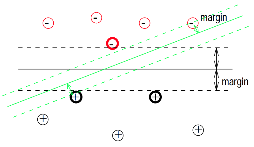
Let’s paint out an example to understand our current position. From looking at the above image, it is clear that there are two types of points. Now, assume that we have model trained and you’re told to choose a specific datapoint within this space. To correctly classify this chosen datapoint, we refer to the fact of which side the datapoint belongs to and then declare a label. Hence, it now safe to say, if we pick the wrong hyperplane from the set of all planes obtained by varying the parameters of the linear model, our prediction will be incorrect. Intuitively the best hyperplane would the mean of all the planes which lies in the centre of both classes. In a general sense, our goal here is to minimise the error of choosing the incorrect hyperplane.

So, anything above the decision boundary should have label $+1$: $x_i$ s.t. $w^Tx_i + b \gt 0$ shall have $y_i = 1$. Similarly, datapoints below the decision boundary should have label$-1$: $x_i$ s.t. $w^Tx_i + b \lt 0$ shall have $y_i = -1$.

This decision boundary can be further condensed as $y(x) = sign(w^Tx_i + b)$. Hence we can verify if an instance is rightly classified by ensuring $y(x) = sign(w^Tx_i + b) \gt 1$.

There is a space between hyperplane and the first elements of each class. We’ll now attempt to classify the elements from these margin such that $w^Tx_i + b = 1$ belongs to the class with label 1 and $w^Tx_i + b = -1$ belongs to the class with label -1.

###Maximising the margin It is clear that the margins are parallel to the hyperplane. This implies the parameters $w^T$ and $b$ apply to the two margins as well. Consider a point $x_i$ on the $w^T + b = -1$. Then a point on $w^T + b = 1$ to $x_i$ is given by $x_2 = x_1 + \lambda w$. The closest point will always lie on the perpendicular to these parallel lines. Vector $\overrightarrow w$ is perpendicular to both lines. So the line segment $\lambda \overrightarrow w$ will be the shortest path connecting points $x_1$ and $x_2$ and the distance between the two points will be $\lambda ||w||$.

Solving for $\lambda$:
$\Rightarrow w^Tx_2 + b = 1$ where $x_2 = x_1 + \lambda w$
$\Rightarrow w^T ( x_1 + \lambda w) + b = 1$ {substituting $x_2 = x_1 + \lambda w$ }
$\Rightarrow w^Tx_1 + \lambda w^Tw + b = 1$
But, w.k.t. $w^T x_1 + b = −1$. We’ll now substituting this in the above equation
$\Rightarrow -1 + \lambda w^Tw = 1$
$\Rightarrow \lambda w^Tw = 2 \Rightarrow \lambda = \frac2{w^Tw} = \frac2{||w||^2}$

Now putting the value of $\lambda$ back in $\lambda||w||$, we have:
$\frac2{||w||^2} ||w|| \Rightarrow \frac2{||w||}\Rightarrow \frac2{\sqrt{ww^T}}$

Clearly, we will try to maximise this distance so that the misclassification error is reduced and thus the datapoints from each class are at the maximum distance. This is the ‘actual margin.’ Thus we must minimise a monotonic function $\frac{ww^T}2$. $\left( \frac2{\sqrt{ww^T}} \Rightarrow \frac{\sqrt{ww^T}}2 \Rightarrow \frac{ww^T}2 \right)$

###Soft and hard margins Suppose in our previous discussions the datapoint were not uniformly distributed, a few were astray, the method of classification would fail to perform due to these outliers. In order to account for this practical behaviour of datapoints we introduce slack variables, $\varepsilon_i \ge 0; \forall x_i$. The reason for introducing a slack variable is to control the degree of flexibility by means of penalties.
$x_i = \begin{cases} on The Correct Side, But Within Or On The Margin Boundary; & \text{p = [0,1)} \\ on The Hyperplane; & \text{p = 1}\\ on The Wrong Side Of The Hyperplane; & \text{p} \gt \text{1} \end{cases}$

We can conveniently formalise this into a quadratic programming problem as below:
$min_{w,b} \frac{ww^T}2 s.t.: y_i(w^T x_i + b) \gt 1 (\forall x_i)$

And with the penalties:
$min_{w,b,\varepsilon_i} \frac{ww^T}2 + \mathbb{C}\sum_i \varepsilon_i s.t.: y_i(w^T x_i + b) \ge 1-\varepsilon_i \text{ }\& \text{ } \varepsilon_i \gt 0 (\forall x_i)$

###Problem of linear separability Many times, mapping $\overrightarrow w$ to a higher dimensional spaces (upto infinity, if required) make them linearly separable whereas they may not linearly separable in their original vector spaces. Consider the mapping $x_i \rightarrow \phi(x_i)$, then the above QP can be re-written as:
$min_{w,b,\varepsilon_i} \frac{ww^T}2 + \mathbb{C}\sum_i \varepsilon_i s.t.: y_i(w^T \phi(x_i) + b) \ge 1-\varepsilon_i \text{ }\& \text{ } \varepsilon_i \gt 0 (\forall x_i)$.

###Lagrangian and Dual Reformulation The technique of Lagrange multipliers captures the idea that in a particular surface in which we need to search for an optimal value, the gradient directions of both the objective and constraint surface must be oriented oppositely. Further to this,
$max_{\alpha_i \ge 0} \text{ } \alpha \left[ 1 − y_i(w^T \phi(x_i) + b)\right]$.

This ensures that when $y_i(w^T \phi(x_i) + b) \ge 1$ the expression above is maximal when $\alpha_i = 0$ as $[1 − y_i(w^T \phi(x_i) + b)]$ is always negative. Otherwise, $y_i(w^T \phi(x_i) +b) < 1$, so $[1−y_i(w^T \phi(x_i) + b)]$ is a positive value, and this expression is maximal when $\alpha_i \rightarrow \infty$. This has the effect of penalising any misclassified datapoints, while assigning 0 penalty to properly classified instances.

This can be captured in:
$min_{w,b}\left[\frac{w^Tw}2 + \sum_i max_{\alpha_i \ge 0}\alpha_i[1 − y_i(w^T \phi(x_i) + b)]\right]$ We now impose a constraint on the Lagrange multipliers$\alpha$ such that $\alpha \not\rightarrow \infty$ and lie within $0 \le \alpha_i \le \mathbb{C}$. This is done to accommodate the slack variables.

A dual problem can be defined as below from the above conditions (that $0 \le \alpha_i \le \mathbb{C}$):
$max_{\alpha \ge 0}[min_{w,b} \mathcal{J}(w, b; α)]$ where $\mathcal{J}\{w,b;\alpha\} = \frac{w^Tw}2 + \sum_i \alpha_i [1 - y_i(w^T \phi(x_i) + b)]$

Clearly, we recognise this as an optimisation problem. By setting $\frac{\partial\mathcal{J}}{\partial w} = 0$ and $\frac{\partial\mathcal{J}}{\partial b} = 0$ we find the optimal setting of $w$ as $\sum_i \alpha_i y_i \phi(x_i)$ and $b$ yields a constraint $\sum_i \alpha_i y_i = 0$ respectively.

Performing a series of mathematical reductions and substitutions, we arrive at:
$min_{w,b}\mathcal{J}(w, b; \alpha) = \sum_i \alpha_i − \frac12 \sum_{i,j} \alpha_i \alpha_j y_i y_j \phi(x_i)^T \phi(x_j)$

Thus the dual form can be written as:
$max_{\alpha \ge 0}\left[\sum_i \alpha_i −\frac12 \sum{i,j}\alpha_i \alpha_j y_i y_j \phi(xi)^T \phi(x_j)\right] s.t. \sum_i \alpha_i y_i = 0 \text{ and } 0 \le \alpha_i \le \mathbb{C}$

###Kernel trick (having very large data points) Assume in order to obtain correct classification results, we had to map the dataset to infinite number of feature vectors, calculating $\phi(x_i)^T \phi(x_j)$ may be intractable. In such situations, the dual enables this as we need to only specify the kernel matrix $K$ containing entries that represent the feature space mapping of 2 features vectors representing 2 datapoints from the dataset. It turns out that the matrix $K$ that operate on the lower dimension vectors $x_i$ and $x_j$ to produce a value equivalent to the dot product of the higher-dimensional vectors. Looking at the original space containing the untransformed dataset, we have constructed a complex non-linear decision boundary. But in order to achieve this, we have to calculate the kernel matrix, $K$. This will lead to a computational overhead provided we use a kernel matrix.

Now, introducing the kernel trick i the dual form, we have:
$max_{\alpha \ge 0}\left[\sum_i \alpha_i −\frac12 \sum_{i,j}\alpha_i \alpha_j y_i y_j K(x_i, x_j)\right]$

###Support Vectors Once we have learned the optimal parameters $\alpha_i$ our task is rather simple. We calculate
$y(x) = sign(w^Tx + b) = \sum_i \alpha_i y_i K(x_i, x) + b$ where $x$ is our instance of a datapoint. $\alpha_i$ is non-zero only for instances $\phi(x_i)$ that lie on or near the decision boundary. These instances are called Support Vector.

###Conclusion If you have scrolled right down here. You have done just right. Look further down and the references may help you understand much better than my attempt. The objective of this post was basically two things. 1. I wanted to write down what I understood about SVMs and 2. I needed an excuse to invest time in learning to typeset using MathJax.

###References: [1] V. Vapnik. The Nature of Statistical Learning Theory. Springer-Verlag, New York, 1995.

[2] CJC Burges. A Tutorial on Support Vector Machines for Pattern Recognition. (PDF)

[3] Nello Cristianini. Support Vector and Kernel Machines. (PDF) ICML Tutorial.

[4] Jason Weston. Support Vector Machine Tutorial. (PDF)